Alternative to captions

According to The Economist, India is held back economically because it has a weak middle class.

The article is 3000 words and has three graphs. How to connect the parts of the text to the appropriate graphs? Numbered captions are one standard technique, but keeping the figure together with a legible caption can be a challenge.

Running the figures inline and referring to them as the next figure or the figure below can work but has issues for multiple columns and page breaks.

A convenient solution is to place a figure number in the chart and use text like (see chart 2).

This works especially well with charts that are largely self documenting.

Compare to expectation

Spotify dominates streaming music, which has been a good thing for the music business.

This domination is even stronger than we might expect. The sizes of top ranked collections, for example the largest cities, are often related by a power law. This observation is called Zipf’s Law.

The number of Spotify subscribers is substantially larger than Zipf predicts.


Use relevant evidence

In October 2017, the Council of Economic Advisers, an agency within the office of the President, released a short report on the effect of a large proposed corporate tax cut on wage growth. The only graphical evidence included is

The presentation is clear, but a graph like this raises the obvious questions: Are these countries similar to the United States? What is significant about these four years?

Presumably the CEA has access to more clearly relevant data.

An analysis by the Economic Policy Institute comes to a very different conclusion. It includes this graph

The evidence is less compelling. You could argue that the 1986 corporate tax cut led to a modest increase in compensation, perhaps through productivity growth. Or perhaps the tax cut interrupted the decades long decline of compensation growth. In any case the United States has not experienced a compensation growth of 2% or more for at least 40 years.

Log scale

Bitcoin is a major phenomenon of out time. There is nothing like very rapid growth to generate excitement.

As is often the case, this linear scale plot obscures rate of change and the small early values. It is worth also looking at a log scale plot.

The early adopters had the best earning potential.

Some people talk about the promise of bitcoin as the new money. Of course this price history shows that it would have been amazingly deflationary. Hardly a good thing.

The price of bitcoin is financial, but its cost is environmental. “Mining” bitcoin takes a huge amount of electricity, and the major mining countries rely heavily on coal fired power plants.

The scale of this electricity consumption can be compared to countries.

The choice of a bar chart is appropriate, as is ordering the countries so that the longest bar is at the bottom, nearest to the scale. The small drop shadows, however, only add blur.

Baseline

The Nikkei 225 recently reached a 21 year high according to The Economist in the October 12, 2017 issue.

The graph is a bit misleading. Because the vertical axis starts at 5000 rather than 0, the index may appear to have tripled since its low rather than doubled.

It is certainly okay to start an axis at a value other than zero for a line graph. But in this case, there is no downside in starting at zero. And our initial impression would be more accurate.

There is another concern: What is special about 1996? Was it a high point?

No.

Including the high point in 1989 would have made a more complete, if longer story.

History and forecast

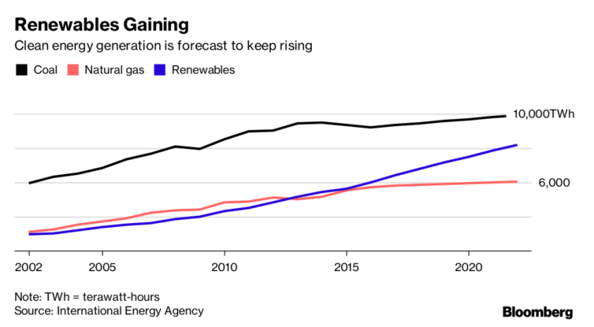
A recent Bloomberg article describes the rapid growth of solar power generation. This graph compares the trend for all renewables to the main fossil fuels used for electricity generation.

The graph is nice and clean. It includes the main message in the title and subtitle. There are only three curves and the have distinct colors. (But shouldn’t the renewables be green?) The axes tick labels are simple, which is adequate since we are not invited to pay attention yearly details.

The graph would be improved if the forecast parts of the curves were indicated. For example using dashes.

China is installing solar capacity much faster than any other country.

The message is well expressed in the subtitle. And it’s a relief that the graph is not a pie chart. The heights of the columns are much easier to compare than the areas of slices would be. The emphasis is on the first and tallest bar, so it does not need to be a different color for emphasis.

Interestingly the article states that the primary motivation in China is concern in the population about air pollution and environmental degradation, while the main driver in the United States is economic.

Prediction bias

“Predictions are hard, especially about the future.” Often attributed to Yoga Berra, it appears that the original author is unknown. (http://quoteinvestigator.com/2013/10/20/no-predict/) Nonetheless, this statement is clearly true.

This graph of world GDP growth contains 42 predictions, almost all too high. This consistent prediction bias does not happen without incentives. The outcome is so consistent that its presenters must believe that optimism is more important than accuracy.

The graph is drawn to show that the 5 year predictions are all 4.5+, when the reality is usually about 3.5. In some cases even the one year predictions are significantly high.

Another way to look at the data is to observe the predictions that are made in any one year. That is to read the graph vertically rather than following the lines. This is another way to see that the predictions for farther in the future are more optimistic.

Including predictions and actuals for years before 2011 would be interesting, even if the graph still begins with 2006. Similarly it would be interesting to see if predictions for years beyond 2017 are still so optimistic.

Source: The predictions were developed by the International Monetary Fund (IMF) and published in their semi-annual World Economic Outlook.

Showing changes

Europe is decreasing CO2 emissions. The United States not so much. And the Europeans will find it difficult to meet their Paris treaty commitment. [The Economist July 8, 2017]

The accompanying chart is relevant but murky.

The chart baseline is 1997, but the treaty reference is 1990. There appears to be little difference between the EU and the US on this scale. China appears to have a huge output but is not mentioned in the article.

Charts that show percent changes from a year are common in finance but can be questionable. Why was that year chosen? Is it representative? Are the series close enough in scale that the comparison makes sense?

The data look like

This graph makes it clearer that the EU is decreasing emissions faster than the US. Also China is clearly not going to achieve a 40% reduction from 1990, but its output is only about twice the US—rather less dramatic than suggested in the original chart.

Data from

Statistics Explained (http://ec.europa.eu/eurostat/statisticsexplained/) – 16/06/2017 and

Source: Boden, T.A., Marland, G., and Andres, R.J. (2017). National CO2 Emissions from Fossil-Fuel Burning, Cement Manufacture, and Gas Flaring: 1751-2014, Carbon Dioxide Information Analysis Center, Oak Ridge National Laboratory, U.S. Department of Energy, doi 10.3334/CDIAC/00001_V2017

A sketch can work

A graph can be good without being dry and sober.

This one has the character of a rough sketch. Yet it communicates better than plain words and has more emotional resonance than a polished graph would. Even without refinements, we have an expectation of how to read a time series plot that works for this example.

The grapher is Charles Hutton, and he’s a hoot.

Interestingly Charles Hutton is also the name of the man credited with inventing contour plots in 1778.

A simple line plot

US airlines have higher fares than European ones. US airlines provide poorer service than European ones. The money goes to profits. The enabling factor is lack of competition. [The Economist April 2017]

Often a simple presentation is best. This line chart shows that dramatic difference in profits and it recent increase.

The Economist uses some conventions that support a clean presentation. The year axis is unlabeled. The vertical variable is identified in a subtitle rather than a vertical axis label. This leads to a compact figure without requiring a sideways label. The character of the chart lines and the wide spacing of the points make a vertical grid unnecessary. The two lines are identified with annotation rather than legend.

The other comparisons in the story are simple pairs of numbers. The Economist has chosen wisely to avoid making these unnecessary bar charts.